Mel Frequency Cepstral Coefficient (MFCC) tutorial

The first step in any automatic speech recognition system is to extract features i.e. identify the components of the audio signal that are good for identifying the linguistic content and discarding all the other stuff which carries information like background noise, emotion etc.

The main point to understand about speech is that the sounds generated by a human are filtered by the shape of the vocal tract including tongue, teeth etc. This shape determines what sound comes out. If we can determine the shape accurately, this should give us an accurate representation of the phoneme being produced. The shape of the vocal tract manifests itself in the envelope of the short time power spectrum, and the job of MFCCs is to accurately represent this envelope. This page will provide a short tutorial on MFCCs.

Mel Frequency Cepstral Coefficents (MFCCs) are a feature widely used in automatic speech and speaker recognition. They were introduced by Davis and Mermelstein in the 1980's, and have been state-of-the-art ever since. Prior to the introduction of MFCCs, Linear Prediction Coefficients (LPCs) and Linear Prediction Cepstral Coefficients (LPCCs) (click here for a tutorial on cepstrum and LPCCs) and were the main feature type for automatic speech recognition (ASR), especially with HMM classifiers. This page will go over the main aspects of MFCCs, why they make a good feature for ASR, and how to implement them.

Steps at a Glance §

We will give a high level intro to the implementation steps, then go in depth why we do the things we do. Towards the end we will go into a more detailed description of how to calculate MFCCs.

1. Frame the signal into short frames.
2. For each frame calculate the periodogram estimate of the power spectrum.
3. Apply the mel filterbank to the power spectra, sum the energy in each filter.
4. Take the logarithm of all filterbank energies.
5. Take the DCT of the log filterbank energies.
6. Keep DCT coefficients 2-13, discard the rest.

There are a few more things commonly done, sometimes the frame energy is appended to each feature vector. Delta and Delta-Delta features are usually also appended. Liftering is also commonly applied to the final features.

Why do we do these things? §

We will now go a little more slowly through the steps and explain why each of the steps is necessary.

An audio signal is constantly changing, so to simplify things we assume that on short time scales the audio signal doesn't change much (when we say it doesn't change, we mean statistically i.e. statistically stationary, obviously the samples are constantly changing on even short time scales). This is why we frame the signal into 20-40ms frames. If the frame is much shorter we don't have enough samples to get a reliable spectral estimate, if it is longer the signal changes too much throughout the frame.

The next step is to calculate the power spectrum of each frame. This is motivated by the human cochlea (an organ in the ear) which vibrates at different spots depending on the frequency of the incoming sounds. Depending on the location in the cochlea that vibrates (which wobbles small hairs), different nerves fire informing the brain that certain frequencies are present. Our periodogram estimate performs a similar job for us, identifying which frequencies are present in the frame.

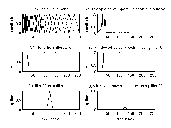
The periodogram spectral estimate still contains a lot of information not required for Automatic Speech Recognition (ASR). In particular the cochlea can not discern the difference between two closely spaced frequencies. This effect becomes more pronounced as the frequencies increase. For this reason we take clumps of periodogram bins and sum them up to get an idea of how much energy exists in various frequency regions. This is performed by our Mel filterbank: the first filter is very narrow and gives an indication of how much energy exists near 0 Hertz. As the frequencies get higher our filters get wider as we become less concerned about variations. We are only interested in roughly how much energy occurs at each spot. The Mel scale tells us exactly how to space our filterbanks and how wide to make them. See below for how to calculate the spacing.

Once we have the filterbank energies, we take the logarithm of them. This is also motivated by human hearing: we don't hear loudness on a linear scale. Generally to double the percieved volume of a sound we need to put 8 times as much energy into it. This means that large variations in energy may not sound all that different if the sound is loud to begin with. This compression operation makes our features match more closely what humans actually hear. Why the logarithm and not a cube root? The logarithm allows us to use cepstral mean subtraction, which is a channel normalisation technique.

The final step is to compute the DCT of the log filterbank energies. There are 2 main reasons this is performed. Because our filterbanks are all overlapping, the filterbank energies are quite correlated with each other. The DCT decorrelates the energies which means diagonal covariance matrices can be used to model the features in e.g. a HMM classifier. But notice that only 12 of the 26 DCT coefficients are kept. This is because the higher DCT coefficients represent fast changes in the filterbank energies and it turns out that these fast changes actually degrade ASR performance, so we get a small improvement by dropping them.

What is the Mel scale? §

The Mel scale relates perceived frequency, or pitch, of a pure tone to its actual measured frequency. Humans are much better at discerning small changes in pitch at low frequencies than they are at high frequencies. Incorporating this scale makes our features match more closely what humans hear.

The formula for converting from frequency to Mel scale is:

To go from Mels back to frequency:

Implementation steps §

We start with a speech signal, we'll assume sampled at 16kHz.

1. Frame the signal into 20-40 ms frames. 25ms is standard. This means the frame length for a 16kHz signal is 0.025*16000 = 400 samples. Frame step is usually something like 10ms (160 samples), which allows some overlap to the frames. The first 400 sample frame starts at sample 0, the next 400 sample frame starts at sample 160 etc. until the end of the speech file is reached. If the speech file does not divide into an even number of frames, pad it with zeros so that it does.

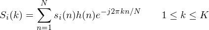
The next steps are applied to every single frame, one set of 12 MFCC coefficients is extracted for each frame. A short aside on notation: we call our time domain signal . Once it is framed we have where n ranges over 1-400 (if our frames are 400 samples) and ranges over the number of frames. When we calculate the complex DFT, we get - where the denotes the frame number corresponding to the time-domain frame. is then the power spectrum of frame .

2. To take the Discrete Fourier Transform of the frame, perform the following:

where is an sample long analysis window (e.g. hamming window), and is the length of the DFT. The periodogram-based power spectral estimate for the speech frame is given by:

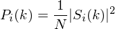
This is called the Periodogram estimate of the power spectrum. We take the absolute value of the complex fourier transform, and square the result. We would generally perform a 512 point FFT and keep only the first 257 coefficents.

3. Compute the Mel-spaced filterbank. This is a set of 20-40 (26 is standard) triangular filters that we apply to the periodogram power spectral estimate from step 2. Our filterbank comes in the form of 26 vectors of length 257 (assuming the FFT settings fom step 2). Each vector is mostly zeros, but is non-zero for a certain section of the spectrum. To calculate filterbank energies we multiply each filterbank with the power spectrum, then add up the coefficents. Once this is performed we are left with 26 numbers that give us an indication of how much energy was in each filterbank. For a detailed explanation of how to calculate the filterbanks see below. Here is a plot to hopefully clear things up:

4. Take the log of each of the 26 energies from step 3. This leaves us with 26 log filterbank energies.

5. Take the Discrete Cosine Transform (DCT) of the 26 log filterbank energies to give 26 cepstral coefficents. For ASR, only the lower 12-13 of the 26 coefficients are kept.

The resulting features (12 numbers for each frame) are called Mel Frequency Cepstral Coefficients.

Computing the Mel filterbank §

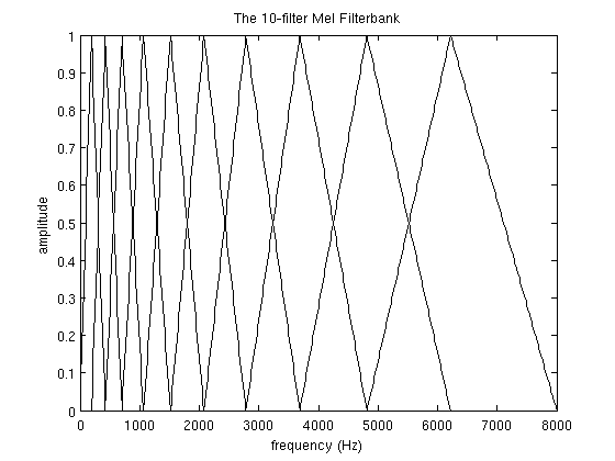
In this section the example will use 10 filterbanks because it is easier to display, in reality you would use 26-40 filterbanks.

To get the filterbanks shown in figure 1(a) we first have to choose a lower and upper frequency. Good values are 300Hz for the lower and 8000Hz for the upper frequency. Of course if the speech is sampled at 8000Hz our upper frequency is limited to 4000Hz. Then follow these steps:

1. Using equation 1, convert the upper and lower frequencies to Mels. In our case 300Hz is 401.25 Mels and 8000Hz is 2834.99 Mels.
2. For this example we will do 10 filterbanks, for which we need 12 points. This means we need 10 additional points spaced linearly between 401.25 and 2834.99. This comes out to:

   m(i) = 401.25, 622.50, 843.75, 1065.00, 1286.25, 1507.50, 1728.74, 
          1949.99, 2171.24, 2392.49, 2613.74, 2834.99

3. Now use equation 2 to convert these back to Hertz:

   h(i) = 300, 517.33, 781.90, 1103.97, 1496.04, 1973.32, 2554.33, 
          3261.62, 4122.63, 5170.76, 6446.70, 8000

   Notice that our start- and end-points are at the frequencies we wanted.
4. We don't have the frequency resolution required to put filters at the exact points calculated above, so we need to round those frequencies to the nearest FFT bin. This process does not affect the accuracy of the features. To convert the frequncies to fft bin numbers we need to know the FFT size and the sample rate,

   f(i) = floor((nfft+1)*h(i)/samplerate)

   This results in the following sequence:

   f(i) =  9, 16,  25,   35,   47,   63,   81,  104,  132, 165,  206,  256

   We can see that the final filterbank finishes at bin 256, which corresponds to 8kHz with a 512 point FFT size.
5. Now we create our filterbanks. The first filterbank will start at the first point, reach its peak at the second point, then return to zero at the 3rd point. The second filterbank will start at the 2nd point, reach its max at the 3rd, then be zero at the 4th etc. A formula for calculating these is as follows:
   
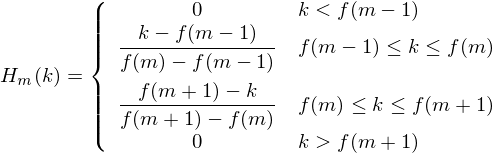
   where is the number of filters we want, and is the list of M+2 Mel-spaced frequencies.

The final plot of all 10 filters overlayed on each other is:

Deltas and Delta-Deltas §

Also known as differential and acceleration coefficients. The MFCC feature vector describes only the power spectral envelope of a single frame, but it seems like speech would also have information in the dynamics i.e. what are the trajectories of the MFCC coefficients over time. It turns out that calculating the MFCC trajectories and appending them to the original feature vector increases ASR performance by quite a bit (if we have 12 MFCC coefficients, we would also get 12 delta coefficients, which would combine to give a feature vector of length 24).

To calculate the delta coefficients, the following formula is used:

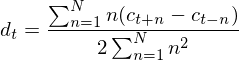
where is a delta coefficient, from frame computed in terms of the static coefficients to . A typical value for is 2. Delta-Delta (Acceleration) coefficients are calculated in the same way, but they are calculated from the deltas, not the static coefficients.

Implementations §

I have implemented MFCCs in python, available here. Use the 'Download ZIP' button on the right hand side of the page to get the code. Documentation can be found at readthedocs. If you have any troubles or queries about the code, you can leave a comment at the bottom of this page.

There is a good MATLAB implementation of MFCCs over here.

References §

Davis, S. Mermelstein, P. (1980) Comparison of Parametric Representations for Monosyllabic Word Recognition in Continuously Spoken Sentences. In IEEE Transactions on Acoustics, Speech, and Signal Processing, Vol. 28 No. 4, pp. 357-366

X. Huang, A. Acero, and H. Hon. Spoken Language Processing: A guide to theory, algorithm, and system development. Prentice Hall, 2001.

Related pages on this site: §

• A tutorial on LPCCs and Cepstrum
• Hidden Markov Model (HMM) tutorial
• Gaussian Mixture Models (GMMs) and the EM Algorithm
• An Intuitive Guide to the Discrete Fourier Transform

comments powered by Disqus