A Tutorial on Cepstrum and LPCCs

The Cepstrum is a sequence of numbers that characterise a frame of speech. The cepstrum computed from the periodogram estimate of the power spectrum can be used in pitch tracking, while the cepstrum computed from the AR power spectral estimate were once used in speech recognition (they have been mostly replaced by MFCCs).

One of the benefits of cepstrum and LPCCs over e.g. LPCs is that you can do cepstral mean subtraction (CMS) on cepstral coefficients to remove channel effects.

Feel free to leave any comments or queries in the comment section down the bottom of this page.

What is the Cepstrum? §

This section will describe the cepstrum computed from the periodogram estimate of the power spectrum. We will first cover autocorrelation a bit, then we will show how the cepstrum is computed in a similar manner. Further on in this article we will cover LPCCs.

The cepstrum can be thought of as being simliar to the autocorrelation sequence. If we have the power spectrum of a signal, we can compute the autocorrelation sequence using the Wiener–Khinchin theorem. In the maths that follows, is the time domain signal, is the complex spectrum, is the power spectrum of and is the autocorrelation sequence of .

By taking the Discrete Fourier Transform of we get the complex spectrum:

If we then take the Inverse Discrete Fourier Transform we get back again:

So far nothing amazing.

BUT, by taking the square of the absolute of the DFT of , we get the power spectrum.

If we take the IDFT of the power spectrum we actually get the Autocorrelation sequence, instead of the original sequence (This is what the Wiener–Khinchin theorem states):

Where does the Cepstrum fit into all this? If we take the log of the power spectrum before the IDFT we actually get the cepstrum:

So you can think of the Cepstrum as a log compressed autocorrelation sequence, as it carries information similar to the autocorrelation sequence (about periodicites in ), but it is computed from the log power spectrum instead of the standard power spectrum.

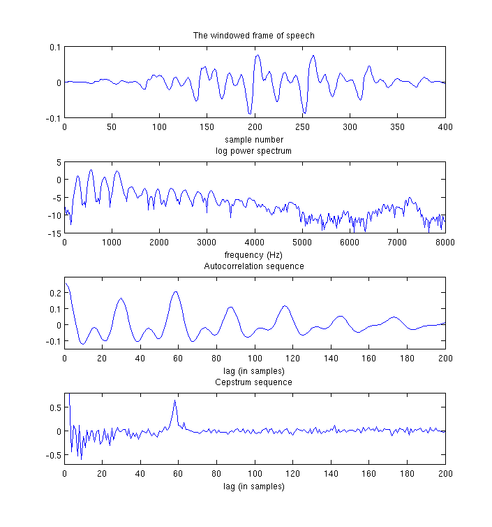
In the figure above you can see the original frame of speech, along with its log power spectrum. The autocorrelation sequence and the cepstrum are also shown. The peak in the cepstrum corresponds to one of the peaks in the autocorrelation sequence, but the peak is much clearer in the cepstrum. This peak is at a lag of 58 samples, this corresponds to a pitch frequency of (16000/58)=275Hz (for a 16kHz signal). This is quite a high pitch frequency, the original speech is from a female speaker. The strong peak is the reason why the cepstrum is often used in pitch tracking applications.

To get the cepstrum in matlab, use the following code:

PowerSpectrum = abs(fft(SpeechFrame,1024)).^2;
AutoCorrelation = ifft(PowerSpectrum,1024);
Cepstrum = ifft(log(PowerSpectrum),1024);

What about LPCCs? §

In the previous section we looked at the standard cepstrum, Linear Prediction Cepstral Coefficients are computed in the same way except they are computed from the smoothed Auto-Regressive power spectrum instead of the periodogram estimate of the power spectrum. For an order 10 AR spectral estimate, the Levinson Durbin algorithm is applied to the first 10 Autocorrelation coefficients to compute 10 linear prediction coefficients. In MATLAB this is done using:

[lp,g] = lpc(frame,10)

The linear prediction coefficients for the frame in the previous section are:

1.00 -2.22  1.68  0.05 -1.28  1.32 -0.30 -0.76  1.35 -1.19  0.44

To compute the cepstrum from the AR spectral estimate, use the following steps:

[lp,g] = lpc(SpeechFrame,10);
ARPowerSpectrum = g ./ abs(fft(lp,1024)).^2;
Cepstrum =  ifft(log(ARPowerSpectrum),1024);

Note that the procedure above is exactly the same as the previous section, only the method for computing the power spectrum is different. The first 10 cepstrum are:

 -11.78  2.22  0.79 -0.12  0.38  0.03 -0.20  0.04 -0.42 -0.11

Computed in this way the first coefficient is ignored, it depends only on g. These are the Linear Prediction Cepstral Coefficients for the frame of speech. If you actually want LPCCs though, don't do it this way, as there is a more efficient way of computing them described in the next section.

The point of this section is to show the relationship between the cepstrum computed from the periodogram power spectrum and LPCCs which are the same except they are computed from the AR estimate of the power spectrum instead.

Computing LPCCs from LPCs §

There is a simple recursive formula for computing Linear Prediction Cepstral Coefficients directly from LPCs without doing any DFTs. In the following equation are the linear prediction coefficients, called lp in the previous section.

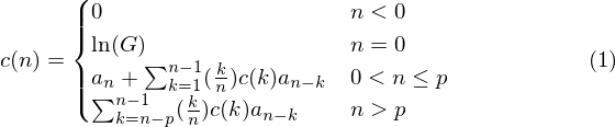
From a finite number of LPC coefficients, an infinite number of cepstral coefficients can be calculated. Research has shown, however, that 12-20 cepstral coefficients are sufficient for speech recognition.

comments powered by Disqus