An Intuitive Discrete Fourier Transform Tutorial

Introduction §

This page will provide a tutorial on the discrete Fourier transform (DFT). It will attempt to convey an understanding of what the DFT is actually doing. Many references exist that specify the mathematics, but it is not always clear what the mathematics actually mean. There are several different ways of understanding the fourier transform, this page will explain it in terms of correlation between a signal and sinusoids of various frequencies.

For a more rigorous explanation of the DFT I can recommend either of these two text books:

• Understanding Digital Signal Processing by Lyons - very readable and good for first timers
• Digital Signal Processing - Principles, Algorithms and Applications by Proakis and Manolakis - more comprehensive but harder to follow without a bit of mathematical maturity

So what is the DFT? It is an algorithm that takes a signal and determines the 'frequency content' of the signal. For the following discussion, a 'signal' is any sequence of numbers, e.g. this is the first 12 numbers of a signal we will look at later (all samples here)

1.00, 0.62, -0.07, -0.87, -1.51, -1.81, -1.70, -1.24, -0.64, -0.15, 0.05, -0.10

We refer to these signals with x(n) where n is the index into the signal. x(0) = 1.00, x(1) = 0.62 etc. Signals such as this arise in many situations, for example all digital audio signals consist of sequences of numbers exactly like the one above. We will consider zero-mean signals, which means if you calculate the mean of the signal you get 0. An explanation for why we do this can be found at the end of the page.

When we try to determine the 'frequency content', we are trying to decompose a complicated signal into simpler parts. Many signals are best described as a sum of many individual frequency components instead of time domain samples. The job of the Discrete Fourier Transform is to determine which frequencies a complicated signal is composed of.

Correlation §

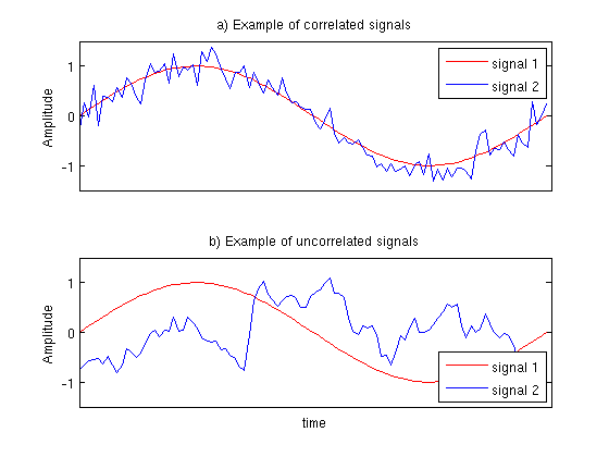
Correlation is a widely used concept in signal processing, which at its heart is a measure of how similar two signals are. If the correlation is high, then the signals are similar, if the correlation is near zero the signals are not very similar. In general, if you ever see an equation that looks like this:

where x and y are signals of some sort, you can say 'Aha! We are calculating the correlation (or similarity) between x and y!'. How does such a simple looking equation calculate the similarity between two signals? If x is very similar to y, then when x(i) is positive, y(i) will also be positive, and when x(i) is negative, y(i) will usually also be negative (since the signals are similar). If we multiply 2 positive numbers (x(i) and y(i)), we get another positive number. If we multiply two negatives, we get another positive number. Then when we sum up all these positive numbers we get a large positive number. What happens if the signals are not very similar? Then sometimes x(i) will be positive while y(i) is negative and vice versa. Other times x(i) will be positive and y(i) will also be positive. In this way when we calculate the final sum we add a few positive numbers and a few negative numbers, which results in a number near zero. This is the idea behind it. Very similar signals will achieve a high correlation, while very different signals will achieve a low correlation, and signals that are a little bit similar will get a correlation score somewhere in between.

Before we go further, I'll mention that correlation can also be negative. This happens when every time x(i) is positive, y(i) is negative and vice versa. This means the result will always be negative (because a negative times a positive is negative). A large negative correlation also means the signals are very similar, but one is inverted with respect to the other.

The Discrete Fourier Transform §

How does Correlation help us understand the DFT? Have a look at the equation for the DFT:

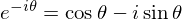
where we sweep k from 0 to N-1 to calculate all the DFT coefficients. When we say 'coefficient' we mean the values of X(k), so X(0) is the first coefficient, X(1) is the second etc. This equation should look very similar to the correlation equation we looked at earlier, because it is calculating the correlation between a signal and a function . But what does it really mean for a signal to be similar to a complex exponential? It makes much more sense if we break up the exponential into sine and cosine components using the following identity:

If we make 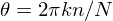, our new DFT equation looks like this:

With a little bit of algebra we can turn it into this:

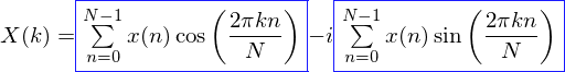
This looks much easier to tackle! It is in fact 2 correlation calculations (each correlation equation is in a blue rectangle), one with a sin wave and another with a cosine. First we calculate the correlation between our signal x(n) and a cosine of a certain frequency, and put the value we get into the real part of X(k). Then we do the same thing with a sine wave, and put the value we get into the imaginary component of X(k).

Correlation with a Cosine §

The next question we wish to ask is how does determining the correlation between a cosine and our signal tell us anything useful? consider a signal of length 100 samples that looks like the following (get the signal samples here)

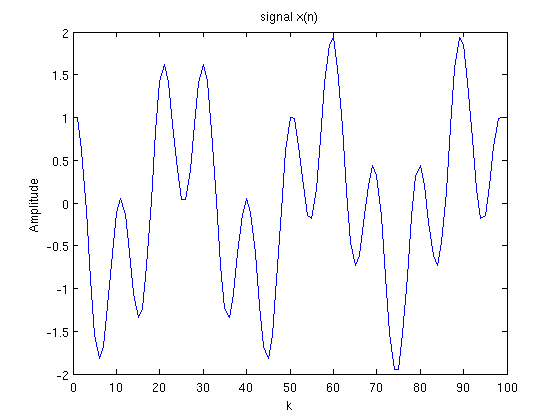
We are going to go through the steps of computing how correlated this signal is with a sequence of cosine and sine waves of increasing frequency. This will be simulating the calculation of the real part of the DFT. Our first calculation will be for k=0 using the equation above:

Here we calculated how correlated the signal is with another signal consisting only of ones (since cos(0) = 1). This turns out to be equal to the sum of the unmodified signal, which from the plot above we see should come out to be close to zero because half the signal looks to be above zero and half below. When we add all of it up the positive components will cancel with the negative components, resulting in a correlation equal to 1.

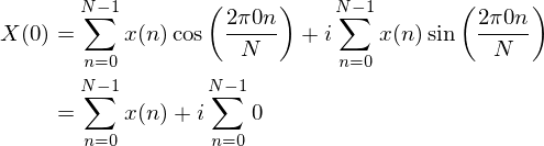
If we set k = 1 we get the following figure: plot(a) has in blue, in red and in black. Plot(b) is , plot (c) is .

The signals in (b) and (c) look like roughly half of the signal is below zero and half above, so when we add up the signals we expect a number near zero. Indeed is equal to 1.0 and is equal to 0, so X(1) is 1+i0.

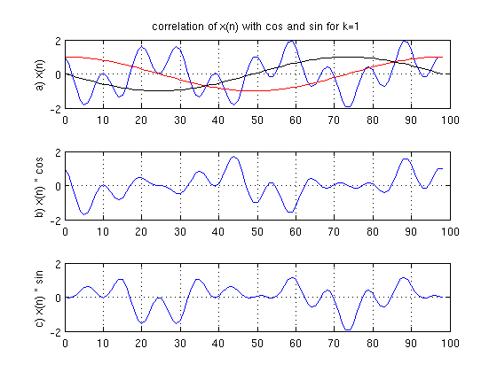
The next figure shows the same signals as the previous, except now k=3. Plot (a) shows x(n) along with the cos and sin waves. Plots (b) and (c) show the product of x(n) with the cos and sin signals respectively.

It is evident that plot (c) is almost entirely positive, with very few negative parts. This means when we sum it up there will be almost no cancellation and we will get a large positive number. In this case the correlation with the cosine comes out to 0, while the correlation with the sin equals 49. This means the DFT coefficient for k = 3 (X(3)) is 0+i49. This process can be continued for each k until the complete DFT is obtained.

Our final discrete Fourier transform looks like this (real part on the left, imaginary part on the right):

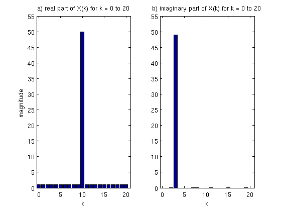
We see that when k=10 we get a peak in the real part (the signal is similar to a cosine), and at k=3 we get a peak in the imaginary part (the signal is similar to a sine). In general though, we don't care if we have a cosine present or a sine, we just want to know if a sinusoid is present, irrespective of phase. To achieve this we combine the real and imaginary components to get the power spectrum:

Note that the power spectrum P(k) has no imaginary component. If we calculate the power spectrum from X(k), we get the following picture:

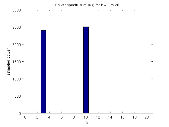
Here we can clearly see that 2 frequencies are present in our signal and little else, which is what we set out to determine.

To convert these values of k into actual frequencies (measured in Hertz), we need the sampling rate of our original signal (fs) and the following formula:

where fs is the sampling frequency and N is the number of samples in our signal (100 for the example above).

Wrapping up §

In an attempt to simplify the discussion I have ignored a few details which I will explain here. I have assumed that all our signals are zero mean, so that the correlation between them is zero when they are dissimilar. This is not necessarily true, but high correlations always mean the signals are similar and lower correlations dissimilar. It is in any case easy enough to subtract the mean from any signals we wish to consider.

In the example above, we calculated the DFT for k = 0 to 20. If we kept calculating coefficients for higher k, we would find that the power spectrum is reflected around N/2. The real part is an even function of k, while the imaginary part is an odd function of k. For further details I'll refer you to the two books recommended at the top of this page.

comments powered by Disqus