Linear Prediction Tutorial
Linear Prediction is one of the simplest ways of predicting future values of a data set. Linear Prediction is of use when you have a time series of data, for example the following points:
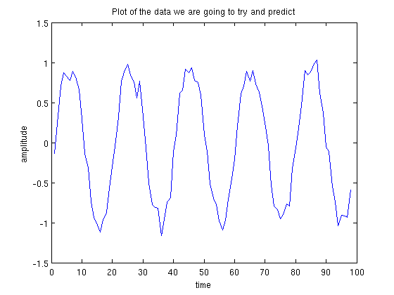
Can we guess what the next number in the sequence should be? What would be a good method for trying to determine it? Somehow we need to use previous data in our time series to predict future samples. In the plot above, we can eye-ball it and guess the next point is going to be around x=-0.3.
Linear Prediction is a method for using previous information to predict the next value in a sequence. We assume we have a chunk of training information which we can learn the sequence behaviour from, then we can apply our learning to situations where the next point is unknown. One of the first things we have to choose when doing linear prediction is the order of our model: this is the number of previous points we use to pedict the next one. If 5 data points are used to predict a sixth, then we call it an order 5 model. We are going to use the data points in the plot above to build an order 5 model that predicts the next point in the series. The first 10 data points are as follows (the whole sequence is available here):
-0.14, 0.24, 0.71, 0.87, 0.83, 0.78, 0.89, 0.82, 0.66, 0.29, -0.14, ...
Remember this is our training information that we are going to use to construct our linear model. A linear model looks like this:

where  are our data points and
  are our linear prediction coefficients. These are the numbers that we have to find. To determine our linear model we look at each sequence of 5 data points and the point that comes after it. For example, the following are all of the length 5 sequences from our set of points:
-0.14, 0.24, 0.71, 0.87, 0.83 -> 0.78
 0.24, 0.71, 0.87, 0.83, 0.78 -> 0.89
 0.71, 0.87, 0.83, 0.78, 0.89 -> 0.82
...
etc.
So the first 5 numbers are -0.14, 0.24, 0.71, 0.87, 0.83, and the sixth is 0.78. So we want values of that satisfy this equation:

we could choose the values of to be pretty much anything. For example, the following values of correctly predict the next point for the equation above:
Unfortunately, these values perform very poorly for predicting all of the other subsequences. We want to find values for that simultaneously perform well on everything. Most of the time it will be impossible to find a set of linear prediction coefficients that always perfectly describe the next point, in this case we want to minimise the error between our predicted value and the actual value. Using a little bit of linear algebra, we can easily solve this problem. Let  be the matrix of all possible length 5 sequences,
  be the vector of linear prediction coefficients and
  be the values we wish to predict. We set up the following equation:

Which we write as:

Now multiply both sides by 
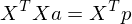
Interestingly  is a toeplitz matrix of Autocorrelation coefficients. Since is a square matrix, we can invert it,

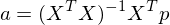
So now we can calculate the vector . Incidentally, 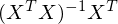 is called the pseudoinverse, which is a very important concept in linear algebra applied to machine learning. Performing the calculation we get:

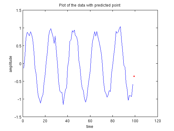
Now we can apply our values of that we have just calculated to predict the next point in the sequence. The last 5 values in our sequence are: -1.04, -0.91, -0.92, -0.93, -0.59. By multiplying them with our values of , we get a value of -0.3016. Below we have a plot showing the data set with the predicted point on the end. It looks pretty good! So we consider this a job well done.
What order model should be chosen? §
Different data requires different order linear models (i.e. different numbers of linear prediction coefficients). How do we know what the best order is? The general rule is that for each sinusoid in the data, you need 2 linear prediction coefficients. For the example above there is a single sinusoid plus some noise, which means an order 2 model would suffice. For speech processing, speech usually has 5 or so dominant frequencies (formants), so an order 10 linear prediction model is often used.
To understand why this is the case, a much deeper understanding of linear prediction and its relationship to poles in autoregressive models is required.
A completely different derivation §
The derivation above is not the one that is given in most books that introduce linear prediction. The end result is the same, but the execution is very different. In this section we will explicitly derive a least squares solution for the values of , and we will see that the result is identical to the example above. I may get around to this derivation at a later date.