Graphically Determining Backpropagation Equations

There has recently been a lot of interest in neural networks, and over time these networks are getting more and more complicated e.g. LSTMs are significantly more complicated than standard feed forward networks. The hardest part about implementing neural networks is figuring out the backpropagation equations to train the weights. This article goes through a simple graphical method for deriving the equations.

The plan is to first introduce the basic rules, then we'll derive the backpropagation equations for a simple feed forward net. Once that is done we'll move on to LSTMs which will give the method a bit of a workout.

The central idea of backpropagation is to determine the error derivative at every point in the network, once the error derivative is known we can figure out how to adjust the weights to minimise the error. Most derivations of backpropagation rely heavily on dense mathematical equations e.g. the UFLDL backprop tutorial. The method we'll go over here is hopefully much easier to figure out.

Many of my writings may lean heavily on 'hand-wavey' ideas, as I always try to understand things intuitively instead of mathematically. There are some people who aren't like that, and thats ok. This is for the people like me. If you find any mistakes, omissions or just know a better way to explain things feel free to leave a comment.

Notation §

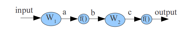
Throughout the equations I use, the values computed through a forward pass of the network (the 'activations') are denoted by lower case letters. The error derivatives are denoted using the delta character i.e. the error derivative at activation is . Note that if is a N by 1 vector, then is a vector of the same size. The error at the output of the network (assuming squared error loss) is:

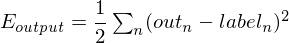
The error derivative is easy to work out:

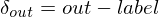
where label is the desired output vector, and out is the actual output vector we get from the network. Remember the whole point of this exercise is to work out the error derivative at each of the weight matrices, so that we can adjust the weight matrices to reduce the error for the next forward pass.

I'll use to denote matrix product and for elementwise product.

The Rules §

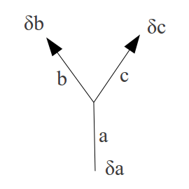
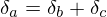
	and	Rule 1: splitting § This case occurs when 1 activation is sent to more than one place, in this case the error derivative at is the sum of the error coming via and the error coming via .
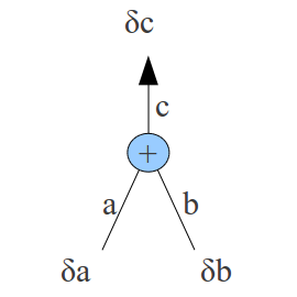
	and	Rule 2: adding § This case occurs when an activation is the sum of two others, in this case the error derivative at is the same as the error at , and the error at is also the same.
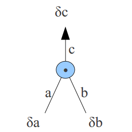
	and .	Rule 3: elementwise multiplication § This case occurs when an activation is the elementwise product of two others, in this case the error derivative at is the product of the error at multiplied by the activation .
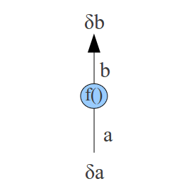
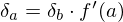
	.	Rule 4: function application § This case occurs when an activation is some function applied to another activation. In this case the error derivative at is the product of the error at and the derivative of the function evaluated at .
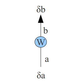
	.	Rule 5: weight matrices § This case occurs when an activation is the product of a matrix with another activation. In effect we are mixing using as the mixing coefficients to get . So to get the error derivative , we need to 'unmix' the error derivative at . Alternatively you can think of it as taking a weighted average of the error derivative at to get the error derivative at , using as our weights.

A simple example §

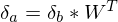
Now that we have the rules, we are going to use them to determine the deltas throughout a simple feedforward 1-hidden layer neural net. First we start of with a nice network diagram of the neural net we will be working with:

In maths:

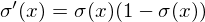
The non-linear functions f() we are using are sigmoids:

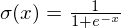
They have a nice derivative which we will be using down below, if:

Our first step is to run the network in forward mode i.e. take an example input and compute the corresponding output. If this is the first pass, initialise the weight matrices with small random numbers. Our output error derivative is :

We can now find using rule 4:

Now we can find using rule 5:

And using rule 4:

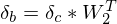
This is all the error derivative calculations done, now we can work out how to update W₁ and W₂ to minimise the error. This part is always the same, once the deltas at the output of a weight matrix are calcluated, the update is always:

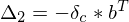
Note the minus signs, because we want to minimise the error we go in the direction of negative gradient. This is the matrix product of the delta at the output of the weight matrix and the input to the weight matrix. Now 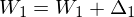and .

To continue, run the forward equation again with the new updated weights, the do backpropagation again. Continue until the error at the output doesn't change much.

Backprop Equations for LSTM RNNs §

The last example was a very simple one, this time we will do something a bit more complex, namely Long Short Term Memory Recurrent Neural Nets or LSTM RNNs for short. Below is shown the network diagram for an LSTM cell.

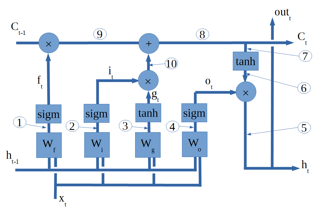
The first step is, once again, to run the network in forward mode. The input will be a D by N matrix where D is the number of dimensions in the input vector, and N is the number of timesteps. The output will be K by N, it can have a different number of dimensions but there has to be the same number of time steps. During the forward pass, all the activations have to be calculated and stored e.g. f_t, output_t etc.

Once we have done the forward pass

comments powered by Disqus