Approximating a function with a polynomial

Polynomial approximation is closely related to interpolation (interpolation is discussed in here). In interpolation, we are given a set of points to fit a polynomial to. We know nothing about the function being interpolated except the values we are given, so we have to use them. However, when approximating a function, we know a lot more and can pick the points we want to use for the interpolating polynomial. The main aim of approximation is not only to find a polynomial that goes through a few points on a function, but we also want the error between our approximating polynomial and the function to be as small as possible.

We are helped in our approximation task by the Weierstrass approximation theorem. It states that every continuous function can be approximated as closely as desired by a polynomial function of sufficient order. This means that no matter what our function is, we will be able to find an approximating polynomial that fits with as little error as we want.

Runge's Phenomenon §

The first example will show you some of the pitfalls that can occur when trying to approximate a function with a polynomial. The function we will try and approximate is between -1 and 1. We will use equidistant points along , then try and fit a polynomial of several different orders to these points.

The points used for this example. This table shows only the points used for the order 5 approximation. The order 12 approximation was performed in the same way.

-1	0
-0.6	0.0133
-0.2	0.6188
0.2	0.6188
0.6	0.133
1	0

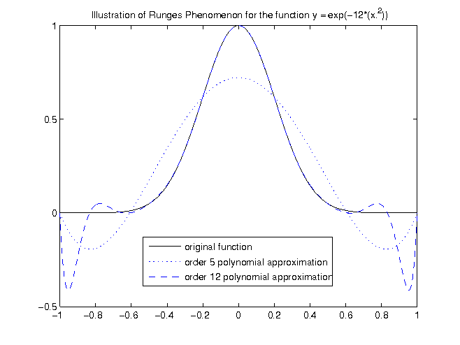
The figure above shows that as we increase the order of the polynomial, our maximum error between and the approximating polynomial is actually increasing near 1 and -1. This increase of error close the edges is known as Runge's Phenomenon. So despite our intuition, where we would expect the error to decrease as we increase the order of our approximating polynomial, we are seeing the opposite. So what can we do? It turns out that the equidistant samples we used to interpolate from are not the best choices for approximation. Since the error becomes largest towards the edges, perhaps we should place more samples near the edges?

Chebyshev Nodes §

So if equidistant nodes are so bad, what can we do to overcome the problem? It turns out that if we sample our function at the 'Chebyshev Nodes', we can geatly decrease the error between the approximating polynomial and the function we are approximating, especially near the edges. It is not important to understand how the nodes are calculated or what they are (they are the roots of the Chebyshev polynomial of the first kind). It is only important to know that they work, and how to calculate them. Assuming we need n points, our values should be:

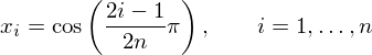
The Chebyshev nodes are only defined over the range , so if we want to use them over a different range we need to scale things a bit. To use them over the range :

The figure below is the exact same problem as that described in the previous section, except now we use samples at the chebyshev nodes, instead of equidistant samples. This table shows only the points used for the order 5 approximation. The order 12 approximation was performed in the same way. The values were calculated using the formula for Chebyshev nodes.

-0.9659	0
-0.7071	0.0025
-0.2588	0.4476
0.2588	0.4476
0.7071	0.0025
0.9659	0

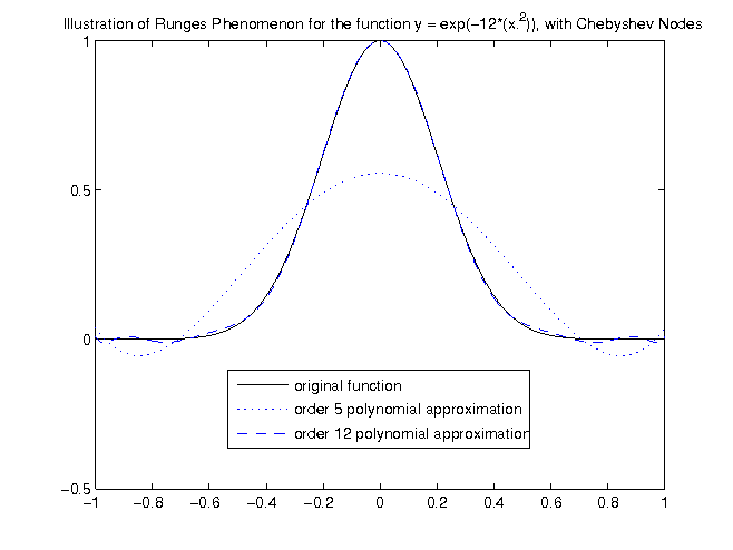
This figure should be compared to the figure exhibiting runge's phenomenon. It is obvious the maximum error near the edges is much smaller in this case. An order 5 polynomial means 6 Chebyshev nodes were chosen between -1 and 1, and the Lagrange method was used to get the approximating polynomial.

The thing to take home from this section is that equidistant samples can be bad for approximation, since increasing the order of the approximating polynomial may increase the error in places (of course there will be situations where this does not happen). When Chebyshev nodes are used, the maximum error is guaranteed to diminish with increasing polynomial order.

The Remez Algorithm §

The Chebyshev nodes are pretty good as far as minimising approximation error. On further thought, it should be obvious that the Chebyshev nodes are not optimal for approximating every function, and that perhaps if we moved some of the nodes around a bit we could get even better approximations. This is where the Remez Algorithm comes in. The Remez Algorithm is an iterative algorithm that starts with the Chebyshev nodes (it can actually have any reasonable starting point, but the Chebyshev nodes are known to be pretty good) and moves them around until the maximum approximation error is minimized. The steps of the algorithm are:

1. A polynomial approximation of the function at the Chebyshev nodes is obtained through Lagrange interpolation.
2. The error between the approximation and the function is calculated. The extrema of the error function are recorded.
3. Solve the N + 2 simultaneous equations (N is the polynomial order): where is the extrema, and and is the polynomial and the error respectively.
4. Solution of step 3 should give new polynomial coefficients. Recalculate the error using these coefficients, and find the extrema of the new error function. Go back to step 3 until converges.

The result is called the polynomial of best approximation, in which the maximum error has been minimised.

Error Comparisons §

This section will compare the error between the original function and the 12th order approximating polynomial. The comparison will be made of error when equidistant nodes (x values) are used, when Chebyshev nodes are used and when the Remez algorithm is used. The error in this case is defined as 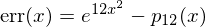, where is the 12th order approximating polynomial.

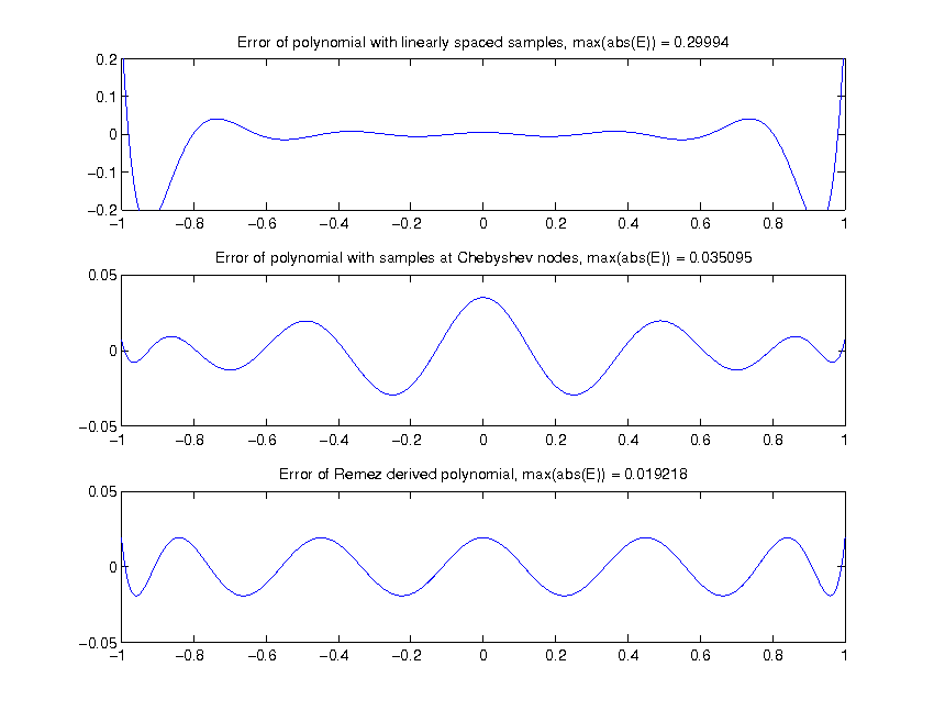
The approximation error using 3 different methods of calculating the approximating polynomial, shown above. The Remez algorithm obviously gives the lowest maximum approximation error. The magnitude of the error is drastically reduced by using Chebyshev Nodes, and reduced even further with the application of the Remez algorithm. To reduce the error further, higher order polynomials can be used. There is however a tradeoff, we use approximations because they are quick to compute, and higher order polynomials take longer to evaluate.

comments powered by Disqus